A UAV data link may look reliable during a short ground test and still fail when the aircraft reaches maximum range, banks, climbs, or carries a high-rate video stream. The difficulty is not simply choosing enough transmit power; every antenna gain, hardware loss, propagation loss, receiver threshold, and operating condition must be evaluated together.
A practical UAV data link budget turns those variables into an estimate of received power and usable margin. The calculation starts with the mission case, follows the RF path from transmitter to receiver, adds flight-related losses, and reveals whether control and payload links retain enough reserve.
Start with the Mission, Not the Formula
Separate the uplink, telemetry, and payload requirements
Command, telemetry, and payload data should not be treated as one generic traffic stream. A command uplink may carry little data but require low latency and very high continuity. Telemetry may tolerate a lower rate, while an HD video downlink can consume most of the available capacity and demand a stronger signal for its selected modulation.
Record the minimum payload throughput, maximum acceptable latency, packet-loss tolerance, and required availability for each service. Use application throughput rather than the radio’s peak physical-layer rate, because protocol overhead, retransmissions, control traffic, and changing modulation reduce the capacity available to the payload. The UAV data link budget should therefore be checked against at least two thresholds: one for maintaining command and control, and another for sustaining the required video or sensor stream.
Choose the worst point in the flight envelope
Distance should represent the weakest realistic point in the route, not merely the advertised mission radius. For an aircraft at a different height from the ground station, use slant range:
Slant range = √(horizontal distance⊃2; + height difference⊃2;)
Geometry alone does not identify the worst point. Banking turns, pitch changes, steep elevation angles, return headings, and payload placement may put the ground station in a weaker part of the airborne antenna pattern. The correct mission input is the position and aircraft attitude that produce the weakest credible link, even when another point is slightly farther away.
Put Every Gain and Loss into One Calculation
Build an input sheet from one actual radio configuration
Start with one complete operating mode. Do not combine the highest transmit power, narrowband sensitivity, widest channel, and maximum data rate when those specifications cannot occur simultaneously.
Input
Unit
Source or basis
Transmitter output power
dBm
Configured RF setting
Transmit antenna gain
dBi
Gain at the actual link angle
Transmit cable and connector loss
dB
Measurement or installation estimate
Operating frequency
MHz
Selected channel
Channel bandwidth
MHz
Selected operating mode
Receive antenna gain
dBi
Gain at the actual elevation and azimuth
Receive-side hardware loss
dB
Feedline, connector, and adapter loss
Receiver sensitivity
dBm
Same bandwidth and modulation being assessed
Additional losses
dB
Orientation, polarization, blockage, and tracking
The units have different roles. dBm expresses an absolute power level, dBi describes antenna gain relative to an isotropic radiator, and dB expresses a gain or loss ratio. Because the equation is logarithmic, gains are added and losses are subtracted directly.
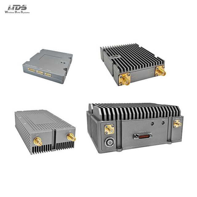
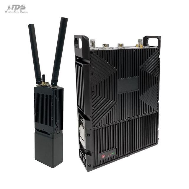
Product specifications must be treated as linked operating conditions. The WDS DDLmesh airborne series supports selectable broadband and narrowband channel widths, adaptive BPSK through 64QAM modulation, adjustable RF output options, 2×2 MIMO functions, and receiver sensitivity of −103 dBm at 5 MHz or −117 dBm at 250 kHz. These values illustrate why the worksheet must select a bandwidth and service rate first: the narrowband sensitivity cannot be used to prove that a broadband video stream will work.
Calculate free-space path loss from frequency and slant range
For an unobstructed point-to-point path, calculate free-space path loss with frequency in MHz and distance in kilometres:
FSPL (dB) = 32.4 + 20 log10(fMHz) + 20 log10(dkm)
Free-space path loss represents a reference condition rather than foliage, terrain diffraction, airframe blockage, interference, or antenna misalignment. Those effects require separate allowances or a more detailed propagation model.
At 2.4 GHz over 10.01 km, the calculation is:
FSPL = 32.4 + 20 log10(2400) + 20 log10(10.01)
FSPL ≈ 120.0 dB
A frequency entered in GHz rather than MHz would produce a 60 dB error with this version of the equation. Units should therefore be shown next to every input cell instead of being left to memory.
Calculate EIRP and predicted received power
Equivalent isotropically radiated power combines the transmit-side terms:
EIRP = Ptx + Gtx − Ltx
If the transmitter produces 30 dBm, the antenna provides 2 dBi in the relevant direction, and the cable path loses 1 dB, the EIRP is 31 dBm. This value should be checked against the rules that apply to the chosen frequency and operating location.
Keep additional losses visible. A single unexplained “safety factor” makes it difficult to determine whether the model includes polarization mismatch, airframe shadowing, tracking error, connector tolerance, or an elevated noise environment. Separate entries also make later flight-test data easier to compare with the original UAV data link budget.
Finally, calculate the air-to-ground and ground-to-air paths in separate columns. They may share the same distance and free-space loss, but different transmit powers, antenna installations, cable runs, bandwidths, and sensitivity thresholds can create significantly different margins.
Decide Whether the Link Still Works in Flight
Compare received power with the right sensitivity value
Receiver sensitivity is not one permanent characteristic of a radio. It normally changes with bandwidth, modulation, coding, target error performance, and sometimes the number of active RF chains. A sensitivity value should only enter the UAV data link budget when it corresponds to the operating mode required by the application.
Calculate the initial link margin as:
Link margin = Predicted received power − Receiver sensitivity
If the predicted signal is −78 dBm and the applicable sensitivity is −103 dBm, the initial margin is 25 dB. That result says the modeled signal is 25 dB above the selected receiver threshold under the assumptions entered into the worksheet.
Reserve margin for changing field conditions
Fade margin is the usable reserve between the expected operating signal and the minimum level required for the selected service. It absorbs losses that vary with time or cannot be predicted precisely during desk-based planning. The required reserve depends on mission criticality, acceptable interruption time, path environment, frequency, antenna behaviour, and the confidence of the input data.
Include allowances for polarization error, connector tolerances, ground-antenna pointing, airframe blockage, partial obstruction, multipath, and installation uncertainty. Interference should be handled carefully because it does not always reduce received signal power; instead, it can raise the effective noise floor and increase the signal level needed for a given data rate. In a simple planning sheet, that effect may be represented as a conservative sensitivity penalty, provided it is clearly labelled.
Fresnel clearance deserves a brief route check for low-altitude paths near terrain, vegetation, buildings, or the ground. Visual line of sight does not guarantee an undisturbed propagation region. Where clearance is questionable, a terrain-aware propagation study is more appropriate than relying on free-space loss alone.
Account for aircraft attitude and antenna pattern
The antenna value in a UAV link calculation should be the gain toward the other radio, not merely the maximum number printed on a datasheet. An omnidirectional antenna in azimuth can still have deep elevation nulls, while installation near carbon fibre, batteries, motors, wiring, cameras, or other antennas can reshape its effective pattern.
Roll, pitch, and yaw therefore belong in the design review. A banked turn may rotate polarization or point a null toward the station, while an overhead pass may place the ground antenna outside the strongest elevation region. The most useful UAV data link budget contains separate scenarios for level flight, maximum bank, climb, overhead transit, and return heading.
MIMO and receive diversity can improve resilience, but the benefit should follow the documented radio mode and installed antenna separation. Spatial multiplexing is primarily used to increase capacity, whereas diversity is intended to improve robustness against fading. Adding an arbitrary “MIMO gain” to received power can overstate performance.
Check both link directions and both performance thresholds
A two-way connection is limited by its weaker direction. The downlink may have higher airborne transmit power and carry heavy video traffic, while the command uplink may use a different ground antenna, channel setting, or sensitivity requirement. Reciprocity of propagation does not make the complete equipment chains identical.
Mission range should be based on whichever threshold is reached first. A UAV may remain controllable after the video stream becomes unusable, but that does not mean the original data-link requirement has been met.
Run a Worked Example, Then Challenge the Result
Complete one realistic UAV data-link calculation
Consider an illustrative 2.4 GHz air-to-ground link with a 10 km horizontal range and a 500 m height difference. The selected radio configuration uses 1 W per RF chain, equivalent to 30 dBm per chain, and a 5 MHz channel with a −103 dBm sensitivity. The example is a calculation exercise rather than a guaranteed range claim.
Budget item
Nominal value
Horizontal range
10.00 km
Height difference
0.50 km
Slant range
10.01 km
Frequency
2,400 MHz
Transmit power
+30 dBm
Airborne antenna gain
+2 dBi
Transmit hardware loss
−1 dB
Free-space path loss
−120 dB
Ground antenna gain
+12 dBi
Receive hardware loss
−1 dB
Predicted received power
−78 dBm
Receiver sensitivity
−103 dBm
Initial link margin
25 dB
The slant range is √(10⊃2; + 0.5⊃2;), or approximately 10.01 km. Free-space loss is about 120 dB, while EIRP is 30 + 2 − 1, or 31 dBm. Received power becomes 30 + 2 − 1 − 120 + 12 − 1 = −78 dBm.
Comparing −78 dBm with −103 dBm leaves 25 dB of nominal margin. That looks workable on paper, but it assumes clear line of sight, accurate antenna gains, no unmodelled installation loss, and receiver sensitivity appropriate to the required service. The opposite-direction calculation must still be completed with its own transmitter, antenna, and receiver values.
Stress-test the budget before approving the design
The nominal result should now be challenged rather than accepted. Suppose a banked turn and airframe placement cause 6 dB of antenna-pattern loss. If interference and implementation uncertainty impose an additional 4 dB equivalent penalty, the available margin falls from 25 dB to approximately 15 dB.
Increasing transmitter power is not always the best first response. Higher RF output can increase electrical load, heat dissipation, system weight, interference, and regulatory exposure, while better antenna placement may recover several decibels without those penalties.
Flight testing should progress from short, low-risk paths to the complete envelope. Record received signal strength, SNR, modulation, throughput, packet loss, and latency during level outbound flight, turns, climbs, overhead passes, and the return heading. Comparing those measurements with the scenario calculations converts the original worksheet into a calibrated model for future missions.
Conclusion
A reliable UAV data link budget should reflect the complete mission rather than an ideal line-of-sight calculation. Checking both link directions, matching receiver sensitivity to the required data rate, and allowing for antenna orientation, interference, and installation losses creates a more realistic basis for design and flight testing.
Shenzhen Sinosun Technology Co., Ltd.’s DDLmesh airborne data-link products can be assessed within this same process, helping teams compare operating configurations and select suitable power, bandwidth, and modulation settings. The result is a clearer path from initial RF planning to dependable command, telemetry, and payload communication.
FAQ
Q: What is a UAV data link budget?
A: A UAV data link budget adds transmitter power and antenna gains, subtracts path and hardware losses, then compares predicted received power with the receiver threshold.
Q: What is the basic RF link budget formula?
A: Predicted received power equals transmitter power plus transmit and receive antenna gains, minus cable, connector, propagation, polarization, blockage, and other implementation losses.
Q: How much link margin does a UAV communication system need?
A: There is no universal target. The required margin depends on mission criticality, frequency, interference, aircraft movement, acceptable outages, and confidence in the propagation assumptions.
Q: Why should slant range be used for UAV link calculations?
A: Slant range reflects the actual three-dimensional distance between the aircraft and ground station, accounting for both horizontal separation and altitude difference.
Q: Should UAV uplink and downlink budgets be calculated separately?
A: Yes. Each direction may use different transmit power, antennas, cable losses, bandwidth, modulation, and receiver sensitivity, producing different operating margins.
Q: Does increasing transmit power always improve UAV link reliability?
A: More power can increase received signal strength, but antenna placement, feeder loss, channel bandwidth, interference, regulatory limits, heat, and energy consumption may be more important.